Raster Modeling and Analysis

Intro

The goal of this lab was to build models showing sand mining suitability and risk in Trempealeau County, WI. To build these models many raster geoprocessing tools were used. After making both the suitability model and the risk model for Trempealeau County, they can be combined to figure out the best locations for sand mining with the smallest impacts on the environment and on the people residing there.

Methods

To make the models for this exercise numerous raster tools and criteria were established. Most commonly the first step would be to convert the feature to a raster so analysis could be performed. If the feature was already a raster then I could skip right to the reclassify step, where the variables were set on classification for that raster. A couple of the other steps required further analysis with tools such as project raster, slope, block statistics, and topo to raster. The combination of all these tools with raster calculator at the end, resulted in the final product for this exercise.

Figure 1. This is the model for the first half of part one of the exercise it consists of making the suitability model for sand mining in Trempealeau County, WI.

Figure 2. The model from the second half of part one shows the workflow for creating a risk model for sand mining in Trempealeau County, WI.

Each objective of the exercise involved working with one different criteria for sand mining. For the suitability model geologic, land use/land cover, distance to railroads, slope, and water-table depth were the criteria looked at to come to the results of the model. This really narrows down the possible locations and allows accurate advice to sand mine owners on where they should operate. It should be noted that the classifications were individually and personally assigned so this shouldn't be used for actual interpretation.
In the second half of the exercise proximity to streams, farmland, residential areas, schools, and the flood plain, and the view from prime recreational areas were the criteria used as a basis for the risk model.

Figure 3. A weighted index model used to weight one of the factors in modeling

For part two of the exercise a weighted index model was used to weigh one of the variables in our models. The variable chosen was supposed to be one that we thought was the most significant and had the biggest effect on sand mining. I chose streams as my largest factor because of the significance of keeping sand mining pollutants out the water.


Results and Discussion

The nine maps below are objectives that were completed in order to find out the risk and suitability of sand mining in Trempealeau County, WI. Each map has either two or three classifications. The classifications are

Green = Suitable
Yellow = Somewhat Suitable
Red = Not Suitable

These colors also allude to the risk of sand mining in the maps that that idea pertains to.
By looking at these maps it becomes clear that the best place for possible sand mining is west central Trempealeau County, although this isn't the only place, just the largest area. Based on my on interpretation it seems the biggest factors in this are the distance to railroad terminals, because there is only one and it is on the far western side. The other big factor I feel is zoning in the county. By looking at the zoning map you can see a large green swathe through the west central part of the county.

             

             

             

Conclusion

Using the knowledge and tools acquired throughout my experience in GIS to complete an exercise like this makes me feel more confident entering the workforce. The advanced raster analysis tools in ArcGIS are very powerful and are a very helpful way to show what needs to be shown. Even though this exercise doesn't hold any real weight as far as classifications, I still feel like it is somewhat accurate to where sand mines would need to be located. It goes to show how much thought can be put into building one of these mines and the implications if all criteria are not met. I think one interesting thing to do would be to use our geocoded mines to see if they follow our suitability and risk models.

Network Analysis for Sand Mines and Rail Terminals

Intro

The goal of this lab was to use network analysis, python scripting, and data flow modeling to carry out the steps of the lab automatically.  This does require some time to set up and get running properly, but after everything runs on its own.  Network analysis is a powerful tool that allows for many different types of routing, in this case to the nearest facility.  Network analysis is a key tool for logistics in many companies and is a smart way to figure out the most efficient route.  Python scripting is another great way to save yourself some time and let the scripts run the tools and create things for you.  Lastly data flow modeling is another piece of the same pie that allows the displaying of a process and then streamlines it.  In this instance we created a python script which narrowed our data by the criteria provided, and created some feature classes.  We then made a data flow model, which we used to run network analysis and provide us with some statistics on the effects of sand trucks on roads.

Methods

First the script was written in python to scale down our data based on criteria.  The criteria were that we didn't want to include any mines that have a railroad loading station, or ones that are within 1.5km of a railroad, because if that's the case they would have built a spur.  Those criteria were met with the script and new feature classes were made based on those criteria.  More information on this part of the lab can be found in my last post.

Network analyst is used to do efficient route modeling.  The network analyst tools were used in this lab to find the nearest facility, the facilities being the rail terminals in Wisconsin, as well as in Winona, MN.  The incidents in the network analyst tool were labeled as incidents.  The data used in the network analysis were from a couple sources.  The network dataset that contains the roads came from ESRI streetmap data, the mine data came from the Wisconsin DNR, and the rail terminal data was provided by the Department of Transportation.

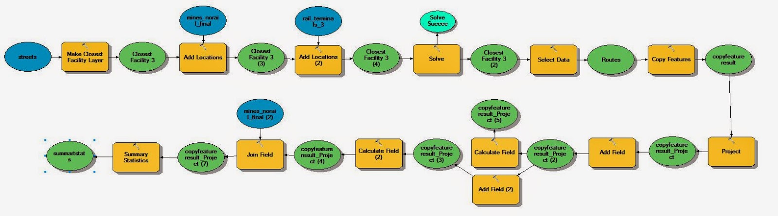
The data flow model used in this lab allowed the automation of the routes, creation of new fields, and also the calculation and summarizing of said fields.  The two fields that were added were "Miles" and "Cost".  To calculate the miles field I took the shape length of each route, which is in meters because of the projection, and divided it by 1,609 (how many meters are in a mile). This equation gave me the number of miles.  In the second calculate field box I calculated the impact in dollars of having sand trucks drive on roads in Wisconsin by county.  The trucks took 50 trips there and back, meaning 100 total trips.  The impact on roads per mile was 2.2 cents. The equation for this calculation was ((100*[Miles])*2.2/100). By dividing the total by 100 I got the number in dollars instead of cents.

Figure 1. The model used in exercise 7 to calculate the impact in dollars on Wisconsin roads.

Results and Discussion

The results shown below are all hypothetical and should not be used to make any decisions regarding policymaking, and should also not be shown in any publications.

Figure 2. Below shows a map of the quickest routes from sand mines to rail terminals.  An observation can be made that some of the routes go into Minnesota and use their roads.  This means there are no impacts on Wisconsin roads, as long as the mine uses the most efficient route.  In these cases it makes more sense economically to use a highway, then stay in Wisconsin and take back roads. As you can see the rail terminals in Wood, Trempealeau, and Chippewa counties have numerous mines that utilize them.  This can be seen in the frequency field of figure 3. What figure 3. also shows is that those three counties mentioned are not the highest on the cost field ranking.  This is due in part to how short the routes are for most of the mines in the counties.  In counties like Burnett and Barron the frequency is lower, but the trips are a lot longer.  Should frac sand mines have to pay for the impacts they have on Wisconsin roads? Should more rail spurs be made to prevent the impact on roads? These are questions that the Wisconsin DOT and the state government will have to ponder as more and more mines become active in the state.

Figure 2. Map of routes from sand mines to rail terminals.

Figure 3. Table of frequency of routes per county as well as cost of trucking on roads by county.

Conclusions

After doing this analysis many questions come to mind on how the state plans to deal with the sand mines, especially since in the coming years there will only be more and more becoming active.  Just by doing this hypothetical exercise one can see the impacts are happening to some degree.  Not to mention the other effects the excessive trucking has like air pollution and noise pollution. network analyst can play a big role in answering some of these questions and will most likely be used when the state does decide to make a decision on this topic.

Python Script for Network Analysis Exercise

Making this python script was part one of exercise seven. In exercise seven we are looking at the effect commercial trucking has on roads from mines to rail stations. To do an analyze of this question we first need to get rid of the mines that have rail spurs and the mines that are not active.  To do this we used python to make a query and acquire our specified results.

The first step was to set the environments for the script and import the system modules.  The workspace was set to our individual exercise seven geodatabase.  The next step was set the variables we would be using in the script, which were just existing feature classes in the geodatabase, as well as some new ones that we would be creating.  The third step was to create three SQL statements that would query out the mines that we wanted.  The first SQL statement selected the active mines, the second statement selected all of the facilities with "Mine" as a type, and lastly the third statement kept out any mines with the word "Rail" in them. The SQL statements were then ran with the addition of the variables created earlier.  The last step was to remove active mines that were within 1.5km of a railroad.  Any closer distance and they likely would have had a spur built to the railroad. To do this the arcpy.SelectLayerByLocation_Management tool was used.  After those parts of the script were done and the script successfully ran, the result was a point feature class containing 41 mines.

Figure 1. The python script used to query active mines with no railroads in a 1.5km radius.